Effective Strategies for Cross-Referencing Values in Multiple Excel Sheets

Quick Links

In Microsoft Excel, it’s a common task to refer to cells on other worksheets or even in different Excel files. At first, this can seem a little daunting and confusing, but once you understand how it works, it’s not so hard.

In this article, we’ll look at how to reference another sheet in the same Excel file and how to reference a different Excel file. We’ll also cover things like how to reference a cell range in a function, how to make things simpler with defined names, and how to use VLOOKUP for dynamic references.

How to Reference Another Sheet in the Same Excel File

A basic cell reference is written as the column letter followed by the row number.

So the cell reference B3 refers to the cell at the intersection of column B and row 3.

When referring to cells on other sheets, this cell reference is preceded with the other sheet’s name. For example, below is a reference to cell B3 on a sheet name “January.”

=January!B3

The exclamation point (!) separates the sheet name from the cell address.

If the sheet name contains spaces, then you must enclose the name with single quotation marks in the reference.

=’January Sales’!B3

To create these references, you can type them directly into the cell. However, it is easier and more reliable to let Excel write the reference for you.

Type an equal sign (=) into a cell, click on the Sheet tab, and then click the cell that you want to cross-reference.

As you do this, Excel writes the reference for you in the Formula Bar.

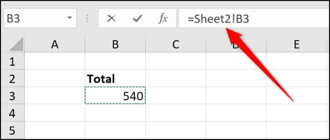
Press Enter to complete the formula.

How to Reference Another Excel File

You can refer to cells of another workbook using the same method. Just be sure that you have the other Excel file open before you begin typing the formula.

Type an equal sign (=), switch to the other file, and then click the cell in that file you want to reference. Press Enter when you’re done.

The completed cross-reference contains the other workbook name enclosed in square brackets, followed by the sheet name and cell number.

=[Chicago.xlsx]January!B3

If the file or sheet name contains spaces, then you’ll need to enclose the file reference (including the square brackets) in single quotation marks.

=’[New York.xlsx]January’!B3

In this example, you can see dollar signs ($) amongst the cell address. This is an absolute cell reference (Find out more about absolute cell references ).

When referencing cells and ranges on different Excel files, the references are made absolute by default. You can change this to a relative reference if required.

If you look at the formula when the referenced workbook is closed, it will contain the entire path to that file.

Although creating references to other workbooks is straightforward, they are more susceptible to issues. Users creating or renaming folders and moving files can break these references and cause errors.

Keeping data in one workbook, if possible, is more reliable.

How to Cross Reference a Cell Range in a Function

Referencing a single cell is useful enough. But you might want to write a function (such as SUM) that references a range of cells on another worksheet or workbook.

Start the function as usual and then click on the sheet and the range of cells—the same way you did in the previous examples.

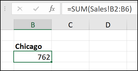
In the following example, a SUM function is summing the values from range B2:B6 on a worksheet named Sales.

=SUM(Sales!B2:B6)

How to Use Defined Names for Simple Cross References

In Excel, you can assign a name to a cell or range of cells. This is more meaningful than a cell or range address when you look back at them. If you use a lot of references in your spreadsheet, naming those references can make it much easier to see what you’ve done.

Even better, this name is unique for all the worksheets in that Excel file.

For example, we could name a cell ‘ChicagoTotal’ and then the cross-reference would read:

=ChicagoTotal

This is a more meaningful alternative to a standard reference like this:

=Sales!B2

It’s easy to create a defined name. Start by selecting the cell or range of cells that you want to name.

Click in the Name Box in the top left corner, type the name you want to assign, and then press Enter.

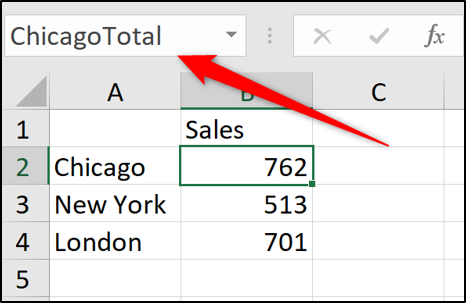
When creating defined names, you cannot use spaces. Therefore, in this example, the words have been joined in the name and separated by a capital letter. You could also separate words with characters like a hyphen (-) or underscore (_).

Excel also has a Name Manager that makes monitoring these names in the future easy. Click Formulas > Name Manager. In the Name Manager window, you can see a list of all of the defined names in the workbook, where they are, and what values they currently store.

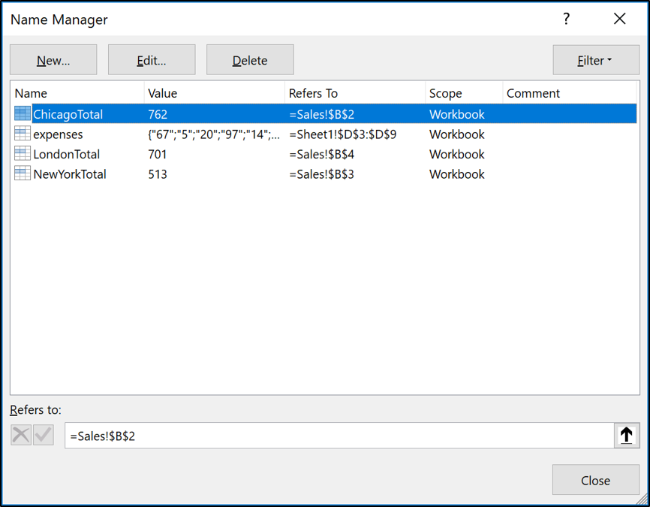
You can then use the buttons along the top to edit and delete these defined names.

How to Format Data as a Table

When working with an extensive list of related data, using Excel’s Format as Table feature can simplify the way that you reference data in it.

Take the following simple table.

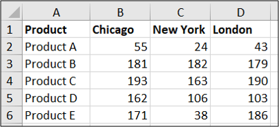
This could be formatted as a table.

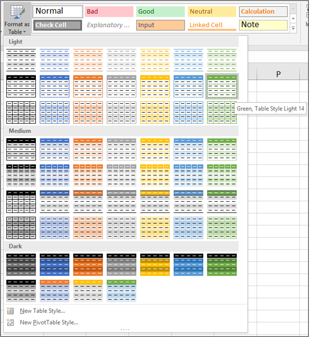
Click on a cell in the list, switch to the “Home” tab, click the “Format as Table” button, and then select a style.

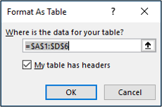
Confirm that the range of cells is correct and that your table has headers.

You can then assign a meaningful name to your table from the “Design” tab.

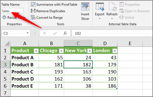
Then, if we needed to sum the sales of Chicago, we could refer to the table by its name (from any sheet), followed by a square bracket ([) to see a list of the table’s columns.

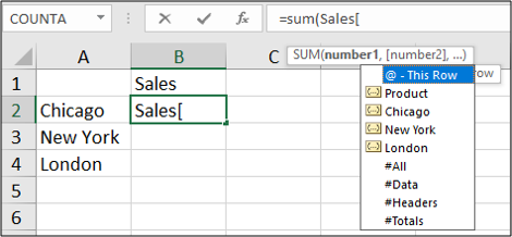
Select the column by double-clicking it in the list and enter a closing square bracket. The resulting formula would look something like this:

=SUM(Sales[Chicago])

You can see how tables can make referencing data for aggregation functions such as SUM and AVERAGE easier than standard sheet references.

This table is small for the purposes of demonstration. The larger the table and the more sheets you have in a workbook, the more benefits you’ll see.

Easy GIF Animator is a powerful animated GIF editor and the top tool for creating animated pictures, banners, buttons and GIF videos. You get extensive animation editing features, animation effects, unmatched image quality and optimization for the web. No other GIF animation software matches our features and ease of use, that’s why Easy GIF Animator is so popular.

How to Use the VLOOKUP Function for Dynamic References

The references used in the examples thus far have all been fixed to a specific cell or range of cells. That’s great and is often sufficient for your needs.

However, what if the cell you are referencing has the potential to change when new rows are inserted, or somebody sorts the list?

In those scenarios, you could not guarantee the value you want will still be in the same cell that you initially referenced.

An alternative in these scenarios is to use a lookup function within Excel to search for the value in a list. This makes it more durable against changes to the sheet.

In the following example, we use the VLOOKUP function to look up an employee on another sheet by their employee ID and then return their start date.

Below is the example list of employees.

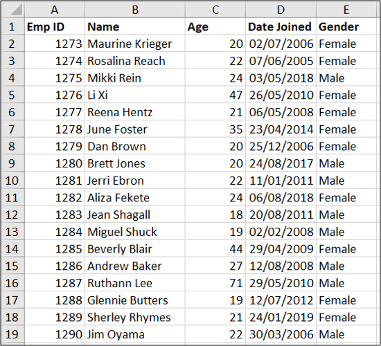
The VLOOKUP function looks down the first column of a table and then returns information from a specified column to the right.

The following VLOOKUP function searches for the employee ID entered into cell A2 in the list shown above and returns the date joined from column 4 (fourth column of the table).

=VLOOKUP(A2,Employees!A:E,4,FALSE)

SwifDoo PDF Perpetual (1 PC) Free upgrade. No monthly fees ever.

Below is an illustration of how this formula searches the list and returns the correct information.

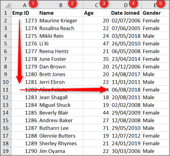
The great thing about this VLOOKUP over the previous examples is that the employee will be found even if the list changes in order.

Note: VLOOKUP is an incredibly useful formula, and we’ve only scratched the surface of its value in this article. You can find out more about how to use VLOOKUP from our article on the subject .

In this article, we have looked at multiple ways to cross-reference between Excel spreadsheets and workbooks. Choose the approach that works for your task at hand, and that you feel comfortable working with.

Win Blog

Effective Strategies for Cross-Referencing Values in Multiple Excel Sheets