
Mastering Data Organization: A Comprehensive Guide to Using Microsoft Excel's Sort Feature

Mastering Data Organization: A Comprehensive Guide to Using Microsoft Excel’s Sort Feature
Quick Links
Key Takeaways
To use the Excel SORT function, insert the following formula into a cell: SORT(range, index, order, by_column). The SORT function will sort your data without disturbing the original data set.
While Microsoft Excel offers a built-in tool for sorting your data, you may prefer the flexibility of a function and formula . We’ll show you how to use the Excel SORT function with helpful examples.
The benefit of using the SORT function is that you can sort the data in a different spot. If you want to manipulate the items without disturbing the original data set, you’ll like the sorting function in Excel. However, if you prefer to sort the items in place, you should use the sort feature instead.
About the Excel SORT Formula
The syntax for the Excel sort formula is
`SORT(range, index, order, by_column)`
where only the first argument is required.
If you’re interested in using the optional arguments, here’s how they work:
- Index : Enter a number to represent the row or column to sort by. Excel sorts by row 1 and column 1 by default.
- Order : Enter 1 for ascending order which is the default if omitted, or -1 for descending order.
- By_colum n: Enter False to sort by row, which is the default if omitted, or True to sort by column. This determines the direction of the sort.
Now, let’s look at examples using the SORT function in Excel.
Use the Excel SORT Function
You can use the SORT function for a range or array in Excel. Again, this does not sort your items in place but in the spot where you enter the formula.
Related: How to List and Sort Unique Values and Text in Microsoft Excel
For a basic example, we’ll simply sort the items in cells A2 through A6 using the defaults for the optional arguments:
=SORT(A2:A6)
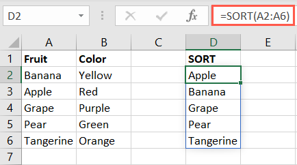
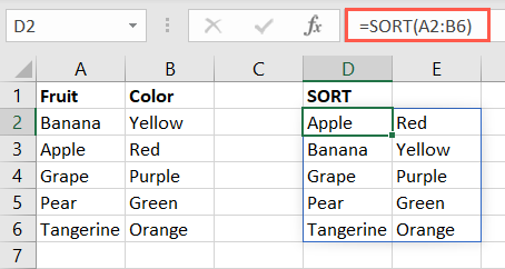
To sort a wider range, we’ll include the cells B2 through B6 as well:
=SORT(A2:B6)
As you can see, the items remain coupled with their attributes.
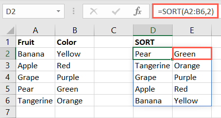
Now we’ll sort our range by the second column rather than the first. So, we enter 2 for the index argument:
=SORT(A2:B6,2)
You can see that our items are sorted in ascending order by the second column, with Green first and Yellow last.
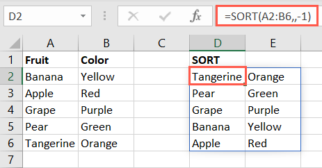
Next, we’ll use an example with the order argument and sort our array in descending order by including -1:
=SORT(A2:B6,,-1)
Notice that we leave the index argument empty because Excel uses the first row and column by default. As intended, we have Tangerine first and Apple last.
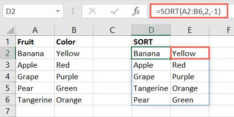
To sort in descending order by the second column, you’d use this formula:
=SORT(A2:B6,2,-1)
Here, we include a 2 for the index argument and a -1 for the order argument. As expected, we see Yellow first and Green last.
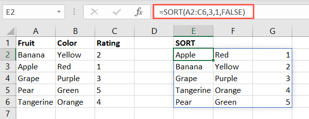
For one final example, we’ll include a value for each argument so you can see how they all work together. We’ll enter a larger array of A2 through C6, a 3 to sort by the third column, a 1 for ascending order, and False for sorting by row direction.
=SORT(A2:C6,3,1,FALSE)
Our items are sorted by the Rating column and, like the other examples above, stay with their attributes.
By using the Excel SORT formula, you can get a different view of your data based on the order you want to see your items. This makes it a handy data analysis tool .
For more, check out how to sort by color or how to sort by date in Excel.
| | Mastering Excel Functions | | |
| —————————- | —————————————————————————————————————————————————————————————————————————————————————————————————————————————————————————————————————————————————————————————————————————————————————————————————————————————————————————————————————————————————————————————————————————————————————————————————————————————————————————————————————————————————————————————————————————————————————————————————————————————————————————————————————————————————————————————————————————————————————————————————————————————————————————————————————————————————————————————————————————————————————————————————————————————————————————————————————————————————————————————————————————————————————————————————————————————————————————————————————————————————————————————————————————————————————————————————————————————————————————————————————————————————————————————————————————————————————————————————————————————————————————————————————————————————————————————————————————————————————————————————————————————————————————————————————— | |
| Functions | AVERAGE · CONCATENATE · COUNT · COUNTIF · DATEDIF · FILTER · FREQUENCY · FV · HYPERLINK · IF · IFS · IMAGE · INDEX · IS · LEN · MATCH ·MEDIAN · RAND · ROUND · RRI · SORT · SQRT · SUBSTITUTE · SUBTOTAL · SUM · SUMIF · TODAY · TRIM · TRUNC · VLOOKUP · WEEKDAY · XLOOKUP · YEAR | |
| Types | Basic · Budgeting · Data Entry · Logical · Text · Time and Date | |
| Explained | Copying Formulas · Evaluating Formulas · Finding Functions · Fixing Formula Errors · Functions vs Formulas · Comparing Lookup Functions · Locking Formulas · Structuring Formulas · Translating Formulas | |
Also read:
- [New] 2024 Approved Real-Time Broadcasts at Your Fingertips Roku and FB Live
- [Updated] Best Screen Reporter Toolkit for YouTube Streamers for 2024
- Beating the Blackout: Expert Tips for League of Legends Display Fixes, 2024 Edition
- Downloading SamFw FRP Tool 3.0 for Honor
- How to Reset Achievements for Steam Games
- Mastering TOTAL WAR SAGA: TROY - Overcoming PC Performance Hiccups & Crashes
- Minecraft Troubles? Conquer the Black Screen Glitch with These Expert Fixes for 2eveRy Gamer
- Optimal Duration for Instagram Content: Understanding the Maximum Length of IG Videos
- Optimizing Performance for Cyberpunk 2077: How to Reduce Excessive CPU Use
- Perfecting YouTube Shorts Step-by-Step Video Production Tips
- Title: Mastering Data Organization: A Comprehensive Guide to Using Microsoft Excel's Sort Feature
- Author: Christopher
- Created at : 2024-12-09 18:46:44
- Updated at : 2024-12-12 19:40:39
- Link: https://win-blog.techidaily.com/mastering-data-organization-a-comprehensive-guide-to-using-microsoft-excels-sort-feature/
- License: This work is licensed under CC BY-NC-SA 4.0.