Step-by-Step Guide: Generating Dummy Data Sets with Microsoft Excel

Quick Links

• Use the Formula Bar
• Adding Random Numbers
• Adding Dates
• Adding Item Data

Creating random data to fill an Excel workbook is as simple as adding a few little-known formulas. These formulas come in handy when honing your Microsoft Excel skills, as they give you fake data to practice with before you risk mistakes with the real thing.

Use the Formula Bar

To start, we’ll enter one of a few formulas in the Formula bar. This is the window below the ribbon, found here.

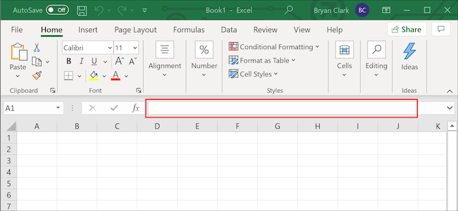
From there, it’s about adding the data you want and then doing a little cleanup.

Adding Random Numbers

To add an integer at random, we’ll use the “RANDBETWEEN” function. Here, we can specify a range of random numerals, in this case, a number from one to 1,000, then copy it to each cell in the column below it.

Click to select the first cell where you’d like to add your random number.

Copy the following formula and paste it into Excel’s Formula bar. You can change the number inside the parenthesis to fit your needs. This formula picks a random number between one and 1,000.

    `=RANDBETWEEN(1,1000)`

Press “Enter” on the keyboard or click the “Green” arrow to apply the formula.

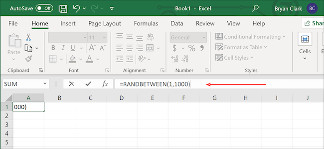
In the lower-right corner, hover over the cell until the “+” icon appears. Click and drag it to the last cell in the column where you want to apply the formula.

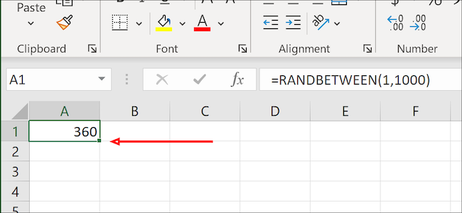
You can use the same formula for monetary values with a simple tweak. By default, RANDBETWEEN only returns whole numbers, but we can change that by using a slightly modified formula. Just change the dates in parenthesis to meet your needs. In this case, we’re choosing a random number between $1 and $1,000.

    `=RANDBETWEEN(1,1000)/100`

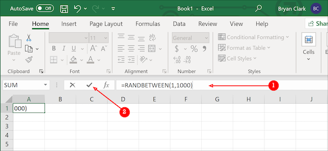
Once done, you’ll need to clean up the data just a little. Start by right-clicking inside the cell, and selecting “Format Cells.”

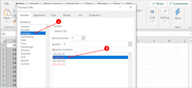
Next, choose “Currency” under the “Category” menu and then select the second option under the “Negative Numbers” option. Press “Enter” on the keyboard to finish.

Adding Dates

Excel’s built-in calendar treats each date as a number, with the number one being January 1, 1900. Finding the number for the date you need isn’t so straightforward, but we’ve got you covered.

Select your starting cell and then copy and paste the following formula into Excel’s Formula bar. You can change anything in parenthesis to fit your needs. Our sample is set to pick a random date in 2020.

    `=RANDBETWEEN(DATE(2020,1,1),DATE(2020,12,31))`

Press “Enter” on the keyboard or click the “Green” arrow to the left of the Formula bar to apply the formula.

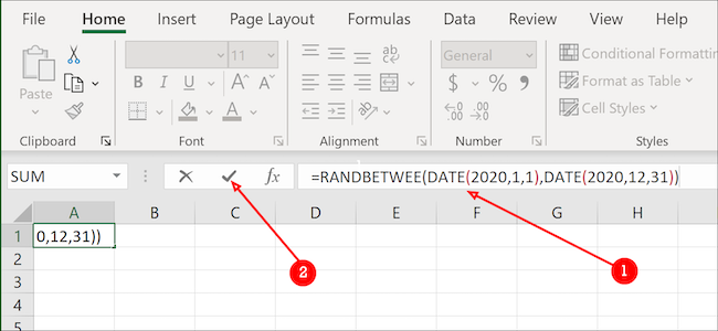
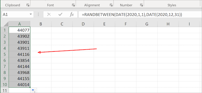
You’ll notice that this doesn’t look anything like a date yet. That’s okay. Just like in the previous section, we’re going to click the “+” sign at the bottom right of the cell and drag it down as far as needed to add additional randomized data.

Once done, highlight all of the data in the column.

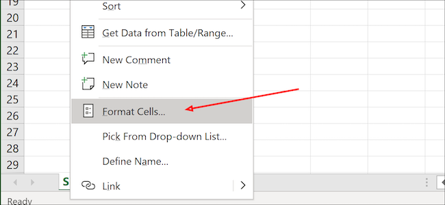
Right-click and select “Format Cells” from the menu.

Click here

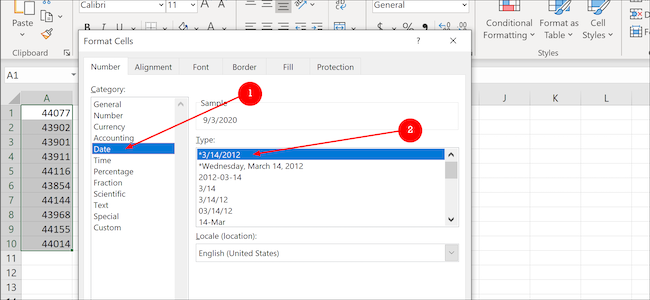
From here, choose the "Date" option and then choose the format you prefer from the available list. Press "OK" once you're done (or "Enter" on the keyboard). Now, all of your random numbers should look like dates.

WonderFox DVD Ripper Pro

Adding Item Data

Randomized data in Excel isn’t limited to just numbers or dates. Using the “VLOOKUP” feature, we can create a list of products, name it, then pull from it to create a randomized list in another column.

To start, we’ll need to create a list of random things. In this example, we’ll add pets from an imaginary pet store starting at cell B2 and ending at B11. You’ll need to number each product in the first column, starting at A2 and ending at A11, coinciding with the product to the right. Hamsters, for example, have the product number 10. The headings in cells A1 and B1 aren’t necessary, though the product numbers and names below them are.

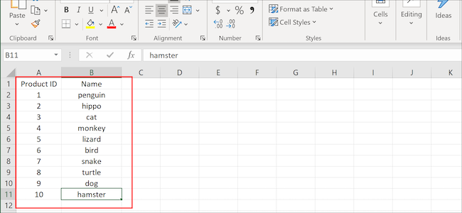
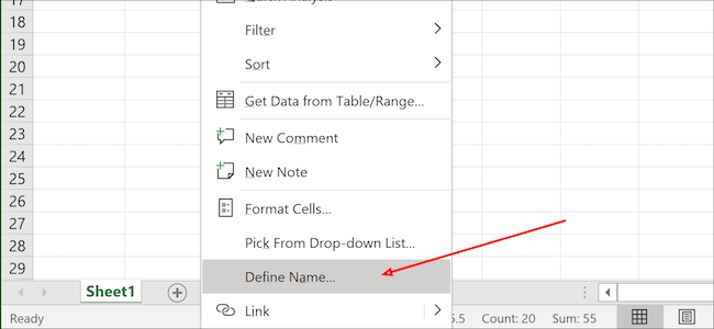
Next, we’ll highlight the entire column, right-click it, and select the “Define Name” option.

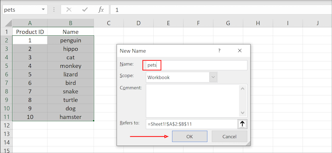
Under “Enter a name for the date range,” we’ll add a name and then click the “OK” button. We’ve now created our list from which to pull random data.

Choose a starting cell and click to highlight it.

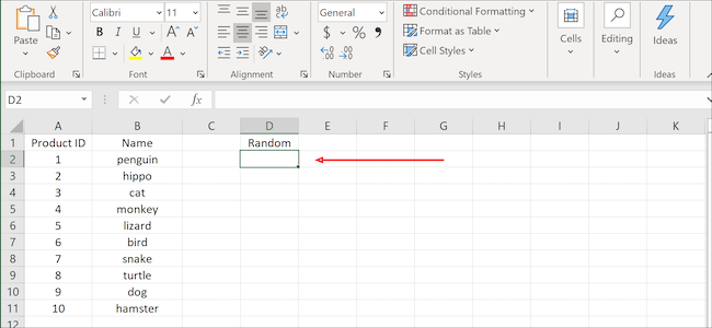
Copy and paste the formula into the Formula bar and then press “Enter” on the keyboard or click the “Green” arrow to apply it. You can change the values (1,10) and the name (“products”) to fit your needs:

    `=VLOOKUP(RANDBETWEEN(1,10),products,2)`

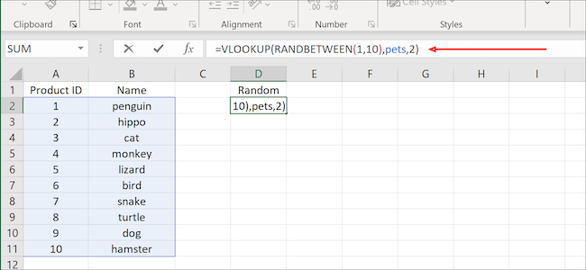
Click and drag the “+” sign at the bottom right of the cell to copy the data into additional cells below (or to the side).

Power Tools add-on for Google Sheets, 12-month subscription

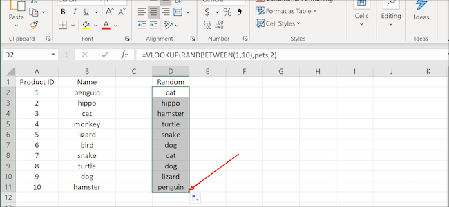
Whether learning pivot tables, experimenting with formatting, or learning how to create a chart for your next presentation, this dummy data could prove to be just what you need to get the job done.