Step-by-Step Guide: Splitting & Extracting Data with Microsoft Excel

Quick Links

• The TEXTBEFORE Function
• The TEXTAFTER Function
• The TEXTSPLIT Function

Microsoft Excel offers a set of functions for working with text . When you want to extract part of a text string or split a string into rows or columns, there are three particular functions that get the job done.

With TEXTBEFORE and TEXTAFTER, you can pull out text before or after a certain word or character. This makes these functions more flexible than the LEFT, RIGHT, and MID functions you might be using. For splitting a string into various cells, you can use TEXTSPLIT.

These three functions are new to Excel as of August 2022. They will roll out to Office Insiders and then all Excel users over time.

The TEXTBEFORE Function

The syntax for the function is

    `TEXTBEFORE(text, delimiter, instance, match_mode, match_end, if_not_found)`

. The first two arguments are required with text being either the actual text or a cell reference and delimiter being the point at which you want the text before.

Here are descriptions of the three optional arguments:

• Instance: Use this argument if there is more than one occurrence of the delimiter in the string and you want a particular one.
• Match_mode: Enter a 0 for case sensitive or 1 for not case sensitive. The default is 0.
• Match_end: Enter 0 to not match the delimiter to the end of the text and 1 to match it. The default is 1.
• If_not_found: Use this argument If you prefer a result rather than an error for values not found.

Now that you know the arguments, let’s look at some example uses for TEXTBEFORE.

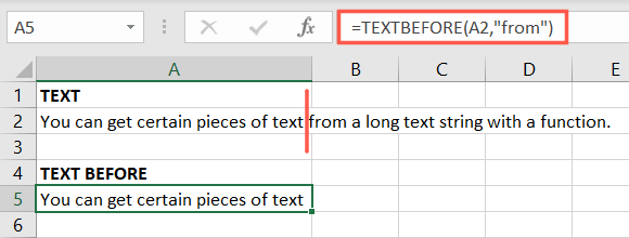
In this first example, we’ll extract all text before the word “from” in cell A2 using this formula:

=TEXTBEFORE(A2,”from”)

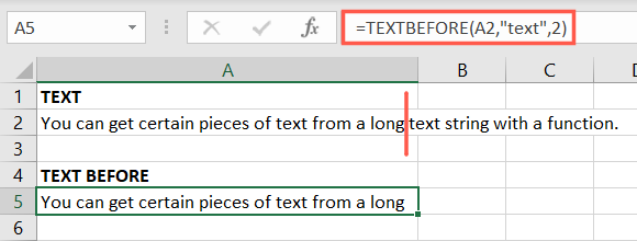
Using this next formula, we’ll extract all text before the second instance of the word “text.”

=TEXTBEFORE(A2,”text”,2)

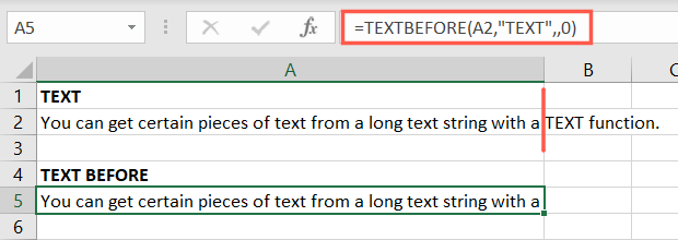
For one more example, we’ll use the match_mode argument for a case-sensitive match.

=TEXTBEFORE(A2,”TEXT”,,0)

Related: 13 Essential Excel Functions for Data Entry

The TEXTAFTER Function

TEXTAFTER is the exact opposite of TEXTBEFORE. The syntax for the function is TEXTAFTER(text, delimiter, instance, match_mode, match_end, if_not_found).

Like its counterpart, the first two arguments are required with text being either the actual text or a cell reference and delimiter being the point at which you want the text after.

The three optional arguments described above also work the same as the TEXTBEFORE function.

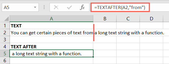
In this first example, we’ll extract all text after the word “from” in cell A2 using this formula:

=TEXTAFTER(A2,”from”)

Using this next formula, we’ll extract all text after the second instance of the word “text.”

=TEXTAFTER(A2,”text”,2)

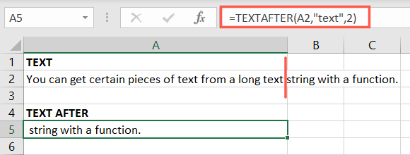
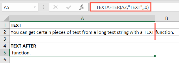
And finally, we’ll use the match_mode argument for a case-sensitive match.

=TEXTAFTER(A2,”TEXT”,,0)

The TEXTSPLIT Function

With the TEXTSPLIT function you can split the text into cells in a row or column based on the delimiter, for example, a space or period.

Related: How to Split Data Into Multiple Columns in Excel

The syntax is TEXTSPLIT(text, column_delimiter, row_delimiter, ignore, match_mode, pad_with) where the first argument is required and can be actual text or a cell reference. By default, the formula splits the text into columns, but you can use rows instead with the row_delimiter argument.

Here are descriptions of the remaining arguments:

• Ignore: Enter FALSE to create an empty cell when two delimiters are consecutive. The default is TRUE.
• Match_mode: Searches the delimiter for a match with the default as case sensitive.
• Pad_with: To pad the result, enter a value. Otherwise, the #N/A error displays.

In this example, we’ll split the text string in cell A2 across columns with a space as our column_delimiter in quotes. Here’s the formula:

=TEXTSPLIT(A2,” “)

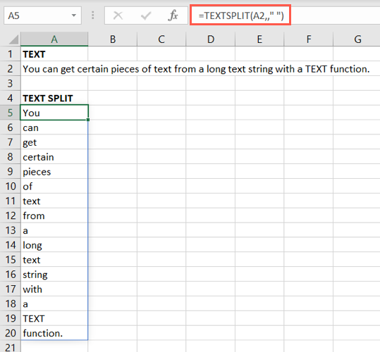
Instead of splitting the string across columns, we’ll split it across rows using a space as our row_delimiter with this formula:

=TEXTSPLIT(A2,,” “)

Notice in this formula, we leave the column_delimiter argument blank and only use the row_delimiter.

Epubor Ultimate for Mac:Helps you read books anywhere, including the best eBook Converter + eBook DRM Removal functions.

For this next example, we’ll split only after the semicolon into another column:

=TEXTSPLIT(A2,”;”)

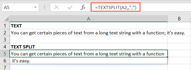
Next, we’ll split only after the semicolon into a row instead of a column:

=TEXTSPLIT(A2,,”;”)

The TEXTSPLIT function is a powerful one. If you’re looking for more complex examples of using the optional arguments, visit the Microsoft Support page for the TEXTSPLIT function .

The next time you want to extract text from a cell or split a long text string, keep these Excel functions in mind. Then, when you need to put strings back together again, learn how to easily add text to a cell with a formula .