
Step-by-Step Tutorial: How to Efficiently Divide Data Using Excel's Split Function

Step-by-Step Tutorial: How to Efficiently Divide Data Using Excel’s Split Function
Quick Links
Do you have multiple values in a single cell that you want to separate into multiple cells? If so, Microsoft Excel has two easy-to-use options to help you split your cells. We’ll show you how to use them.
Table of Contents
Split Cells in Excel With Flash Fill
A quick way to split the values in your cells into multiple cells is by using Excel’s Flash Fill feature . This automatically extracts the values from your cells and puts them into separate multiple cells. To use this feature, you must be running Excel 2013 or later.
To show you how to use this feature, we’ll use the following spreadsheet. In this spreadsheet, we’ll split the names and marks into multiple cells.
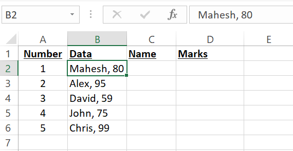
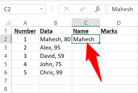
First, click the C2 cell and manually type the name that appears in the B2 cell. In this case, it will be “Mahesh.”
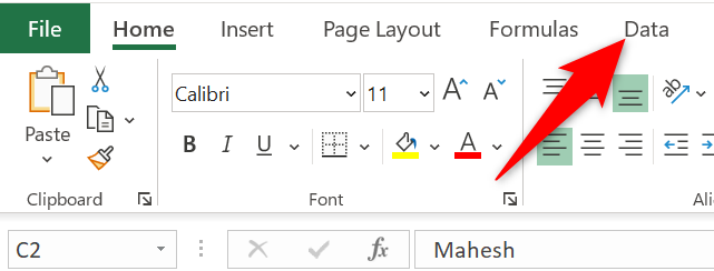
Click the C2 cell so it’s selected. Then, in Excel’s ribbon at the top , click the “Data” tab.
In the “Data” tab, from the “Data Tools” section, select “Flash Fill.”

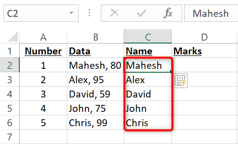
And instantly, Excel will split the names from all the B column records and add those to the C column.
To split the obtained marks, click the D2 cell and manually type the marks for the B2 cell. In this case, it will be “80.”
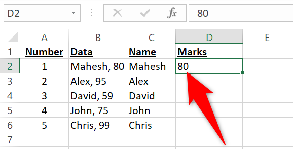
Click the B2 cell so it’s selected. Then, in Excel’s ribbon, click the “Data” tab. Select the “Flash Fill” option and all your marks will be split and be available in the D column.
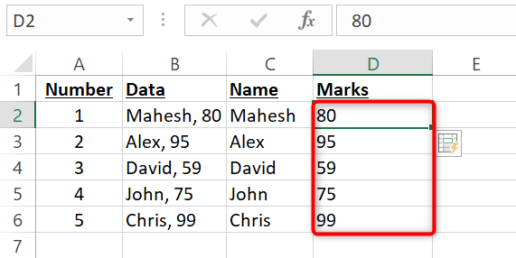
You’re all set. If you’re doing a lot of cell splitting, and you often have to scroll back and forth across your spreadsheet, consider using Excel’s split-screen feature .
Related: How to Use Excel’s Split Screen Function
Split Cells in Excel With Text to Columns
Another way to split cells in Excel is to use the Text to Columns feature . In this feature, you specify what separates your values in your cells, and the feature then uses that separator to split the contents of your cells.
To demonstrate the use of this feature, we’ll again use the same spreadsheet as the above section:

First, in the spreadsheet, click the cells you want to split into multiple cells. Do not select any column headers.
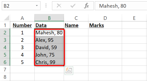
While your cells are selected, in Excel’s ribbon at the top, click the “Data” tab.

In the “Data” tab, from the “Data Tools” section, select the “Text to Columns” option.

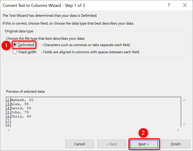
Excel will open a “Text to Columns Wizard” window. Here, choose the “Delimited” option and then click “Next” at the bottom.
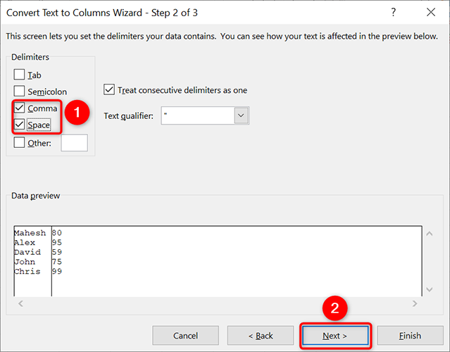
On the next screen, in the “Delimiters” section, select the character or characters that separate the values in your cells. In our example, the values are separated by a comma and a space, so we’ll enable both “Comma” and “Space” options.
On the same “Text to Columns Wizard” window, in the “Data Preview” section, you will see what your data will look like when it’s split into multiple cells. If this looks good to you, then at the bottom of the window, click “Next.”
On the following screen, click the “Destination” field and clear its contents. In the same field, click the up-arrow icon. You will choose where you want to save the split data.
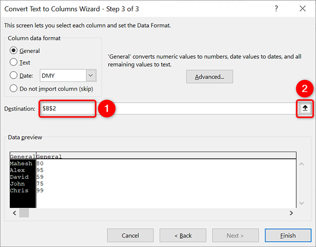
On your spreadsheet, click the C2 cell to store the split data in that cell. Then click the down-arrow icon.

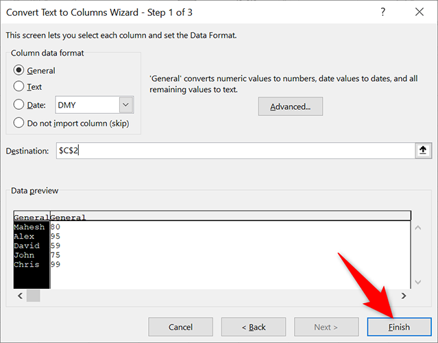
Back on the “Text to Columns Wizard” window, at the bottom, click “Finish.”
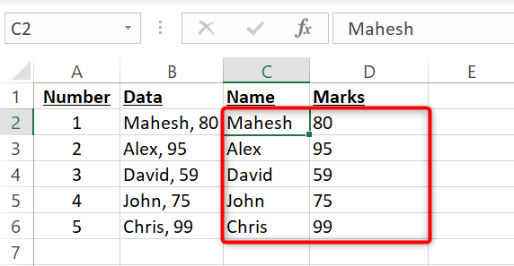
And your single-cell values are now split into multiple cells.
When you’ve got all your data organized how you want it, you may want get insights on it using Excel’s built-in Data Analyzer tool .
Related: How to Use the Analyze Data Feature in Microsoft Excel
Also read:
- [New] 2024 Approved Essential Skills for High-Quality Screen Recordings Using NVIDIA
- [New] Effective Techniques for Screen Display on Google Meet for 2024
- [New] In 2024, ChortleCraft Funny Visuals for Social Engagement
- [Updated] 2024 Approved E-Lecture Documentation
- Battlefield 2042 PC Game Crash Fix - A Comprehensive Guide to Enhancing Performance and Stability
- Effective Fixes for When Your Google Chrome Browser Keeps Crashing at Startup
- Effective Strategies for Protecting Your Active Directory with Windows Server Backup
- Fix Your Gaming Experience: Dead Space Remake Launch Issues Resolved (Updated Guide )
- Frosty Flourishes at the Winter Games
- How to Fix Fallout ^3 Launch Issues - Comprehensive Guide
- Improve Your Fight Against the Titan Quarter in Elden Ring with 6 Quick Tweaks for Better Performance
- In 2024, 4 Methods to Turn off Life 360 On Itel A60 without Anyone Knowing | Dr.fone
- Overcome Lag and Glitches in Modern Warfare 3 - PC Optimization Techniques
- Prevent and Resolve FIFA 22 PC Instability Issues Now
- Revive Your Twitch Viewing Experience: Effective Solutions to Load Failures on the Platform
- Title: Step-by-Step Tutorial: How to Efficiently Divide Data Using Excel's Split Function
- Author: Christopher
- Created at : 2024-12-11 18:00:10
- Updated at : 2024-12-12 16:45:00
- Link: https://win-blog.techidaily.com/step-by-step-tutorial-how-to-efficiently-divide-data-using-excels-split-function/
- License: This work is licensed under CC BY-NC-SA 4.0.