Unlocking Power of INDEX: Effortless Strategies for Data Retrieval in Excel Spreadsheets

Quick Links

• The INDEX Function in Excel
• Use INDEX in Array Form
• Use INDEX in Reference Form

When you need to obtain a value that resides in a particular spot in your spreadsheet, you’ll want one of Excel’s lookup and reference functions. Here, we’ll show you how to find values by location with INDEX in Excel.

You might be creating a complex formula or have values that change often. By using the INDEX function, you designate the cell range along with a row number and column number. Excel locates the value at that intersection and provides the result from the formula.

The INDEX Function in Excel

You can use the INDEX function two different ways in Excel: Array Form and Reference Form.

Array Form provides the value of a certain cell range, or array. Reference Form provides a reference to specific cells and is useful when working with nonadjacent cells.

Let’s look at how to use both.

Use INDEX in Array Form

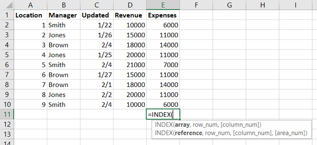
The syntax for the function in Array Form is

    `INDEX(array, row_number, column_number)`

where the first two arguments are required and

    `column_number`

is optional.

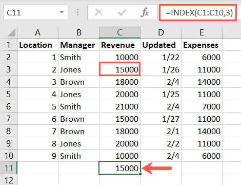
To find the value in the third row in the cell range C1 through C10, you would enter the following formula replacing the cell references with your own.

=INDEX(C1:C10,3)

The number 3 here represents the third row. You don’t need the column number argument because the array is in a single column, C.

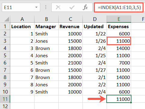
To find the value in the third row and fifth column for the cell range A1 through E10, you would use this formula.

=INDEX(A1:E10,3,5)

Here, the 3 represents the third row and the 5 represents the fifth column. Because the array covers several columns, you should include the column number argument.

Related: How to Number Rows in Microsoft Excel

Use INDEX in Reference Form

The syntax for the function in Reference Form is INDEX(reference, row_number, column_number, area_number) where the first two arguments are required and second two are optional.

You can use a basic formula with the Reference Form of the function as with the Array Form. With the following formula, you receive the value in the third row and fifth column of cells A1 through E10, just like above.

=INDEX(A1:E10,3,5)

So, let’s look at a more robust formula with this form of the INDEX function using nonadjacent cells.

We’re using two cell ranges here, A1 through E4 (first area) and A7 through E10 (second area). To find the value in the third row and fourth column in the first area, you would enter this formula:

=INDEX((A1:E4,A7:E10),3,4,1)

In this formula, you see the two areas, 3 for the third row, 4 for the fourth column, and 1 for the first area A1 through E4.

WinUtilities Pro

To find the value using the same cell ranges, row number, and column number, but in the second area instead of the first, you would use this formula:

=INDEX((A1:E4,A7:E10),3,4,2)

As you can see, everything remains the same except you replace the 1 with a 2 for the second area.

The INDEX function in Excel is a handy one to keep in mind. If you plan to use lookup and reference functions often, be sure to check out how to use VLOOKUP for a range of values and how to use XLOOKUP in Excel .

| | Mastering Excel Functions | | |
| —————————- | —————————————————————————————————————————————————————————————————————————————————————————————————————————————————————————————————————————————————————————————————————————————————————————————————————————————————————————————————————————————————————————————————————————————————————————————————————————————————————————————————————————————————————————————————————————————————————————————————————————————————————————————————————————————————————————————————————————————————————————————————————————————————————————————————————————————————————————————————————————————————————————————————————————————————————————————————————————————————————————————————————————————————————————————————————————————————————————————————————————————————————————————————————————————————————————————————————————————————————————————————————————————————————————————————————————————————————————————————————————————————————————————————————————————————————————————————————————————————————————————————————————————————————————————————————— | |
| Functions | AVERAGE · CONCATENATE · COUNT · COUNTIF · DATEDIF · FILTER · FREQUENCY · FV · HYPERLINK · IF · IFS · IMAGE · INDEX · IS · LEN · MATCH ·MEDIAN · RAND · ROUND · RRI · SORT · SQRT · SUBSTITUTE · SUBTOTAL · SUM · SUMIF · TODAY · TRIM · TRUNC · VLOOKUP · WEEKDAY · XLOOKUP · YEAR | |
| Types | Basic · Budgeting · Data Entry · Logical · Text · Time and Date | |
| Explained | Copying Formulas · Evaluating Formulas · Finding Functions · Fixing Formula Errors · Functions vs Formulas · Comparing Lookup Functions · Locking Formulas · Structuring Formulas · Translating Formulas | |